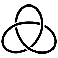
A knot diagram of the trefoil knot
In
topology,
knot theory is the study of
mathematical knots. While inspired by knots which appear in daily life in shoelaces and rope, a mathematician's knot differs in that the ends are joined together so that it cannot be undone. In mathematical language, a knot is an
embedding of a
circle in 3-dimensional
Euclidean space,
R3 (in topology, a circle isn't bound to the classical geometric concept, but to all of its
homeomorphisms). Two mathematical knots are equivalent if one can be transformed into the other via a deformation of
R3 upon itself (known as an
ambient isotopy); these transformations correspond to manipulations of a knotted string that do not involve cutting the string or passing the string through itself.
Knots can be described in various ways. Given a method of description, however, there may be more than one description that represents the same knot. For example, a common method of describing a knot is a planar diagram called a knot diagram. Any given knot can be drawn in many different ways using a knot diagram. Therefore, a fundamental problem in knot theory is determining when two descriptions represent the same knot.
A complete algorithmic solution to this problem exists, which has unknown
complexity. In practice, knots are often distinguished by using a
knot invariant, a "quantity" which is the same when computed from different descriptions of a knot. Important invariants include
knot polynomials,
knot groups, and hyperbolic invariants.
The original motivation for the founders of knot theory was to create a table of knots and
links, which are knots of several components entangled with each other. Over six billion knots and links have been tabulated since the beginnings of knot theory in the 19th century.
History[edit]
Archaeologists have discovered that knot tying dates back to prehistoric times. Besides their uses such as
recording information and
tying objects together, knots have interested humans for their aesthetics and spiritual symbolism. Knots appear in various forms of Chinese artwork dating from several centuries BC (see
Chinese knotting). The
endless knotappears in
Tibetan Buddhism, while the
Borromean rings have made repeated appearances in different cultures, often representing strength in unity. The
Celtic monks who created the
Book of Kells lavished entire pages with intricate
Celtic knotwork.
A mathematical theory of knots was first developed in 1771 by Alexandre-Théophile Vandermonde who explicitly noted the importance of topological features when discussing the properties of knots related to the geometry of position. Mathematical studies of knots began in the 19th century with Gauss, who defined the linking integral (Silver 2006). In the 1860s, Lord Kelvin's theory that atoms were knots in the aether led to Peter Guthrie Tait's creation of the first knot tables for complete classification. Tait, in 1885, published a table of knots with up to ten crossings, and what came to be known as the Tait conjectures. This record motivated the early knot theorists, but knot theory eventually became part of the emerging subject of topology.
These topologists in the early part of the 20th century—
Max Dehn,
J. W. Alexander, and others—studied knots from the point of view of the
knot group and invariants from
homology theory such as the
Alexander polynomial. This would be the main approach to knot theory until a series of breakthroughs transformed the subject.
In the last several decades of the 20th century, scientists became interested in studying
physical knots in order to understand knotting phenomena in
DNA and other polymers. Knot theory can be used to determine if a molecule is
chiral(has a "handedness") or not (
Simon 1986).
Tangles, strings with both ends fixed in place, have been effectively used in studying the action of
topoisomerase on DNA (
Flapan 2000). Knot theory may be crucial in the construction of quantum computers, through the model of
topological quantum computation (
Collins 2006).
Knot equivalence[edit]
On the left, the unknot, and a knot equivalent to it. It can be more difficult to determine whether complex knots, such as the one on the right, are equivalent to the unknot.
A knot is created by beginning with a one-
dimensional line segment, wrapping it around itself arbitrarily, and then fusing its two free ends together to form a closed loop (
Adams 2004) (
Sossinsky 2002). Simply, we can say a knot

is an
injective and
continuous function ![K:[0,1]\to \mathbb{R}^3](https://upload.wikimedia.org/math/8/a/a/8aa0077e4780baa9ea82e0f17c1a11f6.png)
with

. When topologists consider knots and other entanglements such as
links and
braids, they consider the space surrounding the knot as a viscous fluid. If the knot can be pushed about smoothly in the fluid, without intersecting itself, to coincide with another knot, the two knots are considered equivalent. The idea of
knot equivalence is to give a precise definition of when two knots should be considered the same even when positioned quite differently in space. A formal mathematical definition is that two knots

are equivalent if there is an
orientation-preserving homeomorphism 
with

, and this is known as an
ambient isotopy.
The basic problem of knot theory, the
recognition problem, is determining the equivalence of two knots.
Algorithms exist to solve this problem, with the first given by
Wolfgang Haken in the late 1960s (
Hass 1998). Nonetheless, these algorithms can be extremely time-consuming, and a major issue in the theory is to understand how hard this problem really is (
Hass 1998). The special case of recognizing the
unknot, called the
unknotting problem, is of particular interest (
Hoste 2005).
Knot diagrams[edit]
A useful way to visualise and manipulate knots is to project the knot onto a plane—think of the knot casting a shadow on the wall. A small change in the direction of projection will ensure that it is
one-to-one except at the double points, called
crossings, where the "shadow" of the knot crosses itself once transversely (
Rolfsen 1976). At each crossing, to be able to recreate the original knot, the over-strand must be distinguished from the under-strand. This is often done by creating a break in the strand going underneath. The resulting diagram is an
immersed plane curve with the additional data of which strand is over and which is under at each crossing. (These diagrams are called
knot diagrams when they represent a
knot and
link diagrams when they represent a
link.) Analogously, knotted surfaces in 4-space can be related to
immersed surfaces in 3-space.
A
reduced diagram is a knot diagram in which there are no
reducible crossings (also
nugatory or
removable crossings), or in which all of the reducible crossings have been removed.(
Weisstein, ReducedKnotDiagram)(
Weisstein, ReducibleCrossing)
Reidemeister moves[edit]
In 1927, working with this diagrammatic form of knots,
J. W. Alexander and G. B. Briggs, and independently
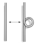
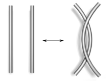
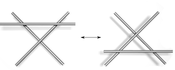
Kurt Reidemeister, demonstrated that two knot diagrams belonging to the same knot can be related by a sequence of three kinds of moves on the diagram, shown below. These operations, now called the
Reidemeister moves, are:
- Twist and untwist in either direction.
- Move one strand completely over another.
- Move a strand completely over or under a crossing.
Reidemeister moves
  |  |
| Type I | Type II |
 |
| Type III |
The proof that diagrams of equivalent knots are connected by Reidemeister moves relies on an analysis of what happens under the planar projection of the movement taking one knot to another. The movement can be arranged so that almost all of the time the projection will be a knot diagram, except at finitely many times when an "event" or "catastrophe" occurs, such as when more than two strands cross at a point or multiple strands become tangent at a point. A close inspection will show that complicated events can be eliminated, leaving only the simplest events: (1) a "kink" forming or being straightened out; (2) two strands becoming tangent at a point and passing through; and (3) three strands crossing at a point. These are precisely the Reidemeister moves (
Sossinsky 2002, ch. 3) (
Lickorish 1997, ch. 1).
Knot invariants[edit]
Main article:
Knot invariant
A knot invariant is a "quantity" that is the same for equivalent knots (
Adams 2004)(
Lickorish 1997)(
Rolfsen 1976). For example, if the invariant is computed from a knot diagram, it should give the same value for two knot diagrams representing equivalent knots. An invariant may take the same value on two different knots, so by itself may be incapable of distinguishing all knots. An elementary invariant is
tricolorability.
Knot polynomials[edit]
The Alexander–Conway polynomial is actually defined in terms of
links, which consist of one or more knots entangled with each other. The concepts explained above for knots, e.g. diagrams and Reidemeister moves, also hold for links.
Consider an oriented link diagram,
i.e. one in which every component of the link has a preferred direction indicated by an arrow. For a given crossing of the diagram, let

be the oriented link diagrams resulting from changing the diagram as indicated in the figure:
The original diagram might be either

or

, depending on the chosen crossing's configuration. Then the Alexander–Conway polynomial,
C(
z), is recursively defined according to the rules:
- C(O) = 1 (where O is any diagram of the unknot)

The second rule is what is often referred to as a
skein relation. To check that these rules give an invariant of an oriented link, one should determine that the polynomial does not change under the three Reidemeister moves. Many important knot polynomials can be defined in this way.
The following is an example of a typical computation using a skein relation. It computes the Alexander–Conway polynomial of the
trefoil knot. The yellow patches indicate where the relation is applied.
- C(
 ) = C(
 ) + z C(
 )
)
gives the unknot and the
Hopf link. Applying the relation to the Hopf link where indicated,
- C(
 ) = C(
 ) + z C(
 )
)
gives a link deformable to one with 0 crossings (it is actually the
unlink of two components) and an unknot. The unlink takes a bit of sneakiness:
- C(
 ) = C(
 ) + z C(
 )
)
which implies that C(unlink of two components) = 0, since the first two polynomials are of the unknot and thus equal.
Putting all this together will show:
- C(trefoil) = 1 + z(0 + z) = 1 + z2.
Since the Alexander–Conway polynomial is a knot invariant, this shows that the trefoil is not equivalent to the unknot. So the trefoil really is "knotted".
The left handed trefoil knot.
The right handed trefoil knot.
Actually, there are two trefoil knots, called the right and left-handed trefoils, which are
mirror images of each other (take a diagram of the trefoil given above and change each crossing to the other way to get the mirror image). These are not equivalent to each other, meaning that they are not amphicheiral. This was shown by
Max Dehn, before the invention of knot polynomials, using group theoretical methods (
Dehn 1914). But the Alexander–Conway polynomial of each kind of trefoil will be the same, as can be seen by going through the computation above with the mirror image. The
Jonespolynomial can in fact distinguish between the left and right-handed trefoil knots (
Lickorish 1997).
Hyperbolic invariants[edit]
The
Borromean rings are a link with the property that removing one ring unlinks the others.
SnapPea's cusp view: the
Borromean ringscomplement from the perspective of an inhabitant living near the red component.
Geometry lets us visualize what the inside of a knot or link complement looks like by imagining light rays as traveling along the
geodesics of the geometry. An example is provided by the picture of the complement of the
Borromean rings. The inhabitant of this link complement is viewing the space from near the red component. The balls in the picture are views of
horoball neighborhoods of the link. By thickening the link in a standard way, the horoball neighborhoods of the link components are obtained. Even though the boundary of a neighborhood is a torus, when viewed from inside the link complement, it looks like a sphere. Each link component shows up as infinitely many spheres (of one color) as there are infinitely many light rays from the observer to the link component. The fundamental parallelogram (which is indicated in the picture), tiles both vertically and horizontally and shows how to extend the pattern of spheres infinitely.
This pattern, the horoball pattern, is itself a useful invariant. Other hyperbolic invariants include the shape of the fundamental paralleogram, length of shortest geodesic, and volume. Modern knot and link tabulation efforts have utilized these invariants effectively. Fast computers and clever methods of obtaining these invariants make calculating these invariants, in practice, a simple task (
Adams, Hildebrand & Weeks 1991).
Higher dimensions[edit]
A knot in three dimensions can be untied when placed in four-dimensional space. This is done by changing crossings. Suppose one strand is behind another as seen from a chosen point. Lift it into the fourth dimension, so there is no obstacle (the front strand having no component there); then slide it forward, and drop it back, now in front. Analogies for the plane would be lifting a string up off the surface, or removing a dot from inside a circle.
In fact, in four dimensions, any non-intersecting closed loop of one-dimensional string is equivalent to an unknot. First "push" the loop into a three-dimensional subspace, which is always possible, though technical to explain.
Knotting spheres of higher dimension[edit]
Since a knot can be considered topologically a 1-dimensional sphere, the next generalization is to consider a
two-dimensional sphere embedded in a four-dimensional ball. Such an embedding is unknotted if there is a homeomorphism of the 4-sphere onto itself taking the 2-sphere to a standard "round" 2-sphere.
Suspended knots and
spun knots are two typical families of such 2-sphere knots.
The mathematical technique called "general position" implies that for a given
n-sphere in the
m-sphere, if
m is large enough (depending on
n), the sphere should be unknotted. In general,
piecewise-linear n-spheres form knots only in (
n + 2)-space (
Zeeman 1963), although this is no longer a requirement for smoothly knotted spheres. In fact, there are smoothly knotted (4
k − 1)-spheres in
6k-space, e.g. there is a smoothly knotted 3-sphere in the 6-sphere (
Haefliger 1962)(
Levine 1965). Thus the codimension of a smooth knot can be arbitrarily large when not fixing the dimension of the knotted sphere; however, any smooth
k-sphere in an
n-sphere with 2
n − 3
k − 3 > 0 is unknotted. The notion of a knot has further generalisations in mathematics, see:
knot (mathematics),
isotopy classification of embeddings.
An
n-knot is a single
Sn embedded in
Sm. An
n-link is
k-copies of
Sn embedded in
Sm, where
k is a natural number. Both the
m =
n + 2 case and the
m >
n + 2 case are researched well. The
n > 1 case has different futures from the
n = 1 case and is an exciting field.
[1] [2]
Adding knots[edit]
Two knots can be added by cutting both knots and joining the pairs of ends. The operation is called the
knot sum, or sometimes the
connected sum or
composition of two knots. This can be formally defined as follows (
Adams 2004): consider a planar projection of each knot and suppose these projections are disjoint. Find a rectangle in the plane where one pair of opposite sides are arcs along each knot while the rest of the rectangle is disjoint from the knots. Form a new knot by deleting the first pair of opposite sides and adjoining the other pair of opposite sides. The resulting knot is a sum of the original knots. Depending on how this is done, two different knots (but no more) may result. This ambiguity in the sum can be eliminated regarding the knots as
oriented, i.e. having a preferred direction of travel along the knot, and requiring the arcs of the knots in the sum are oriented consistently with the oriented boundary of the rectangle.
The knot sum of oriented knots is
commutative and
associative. A
knot is prime if it is non-trivial and cannot be written as the knot sum of two non-trivial knots. A knot that can be written as such a sum is
composite. There is a prime decomposition for knots, analogous to
prime and composite numbers (
Schubert 1949). For oriented knots, this decomposition is also unique. Higher-dimensional knots can also be added but there are some differences. While you cannot form the unknot in three dimensions by adding two non-trivial knots, you can in higher dimensions, at least when one considers
smoothknots in codimension at least 3.
Tabulating knots[edit]
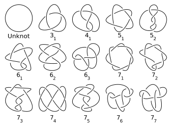
A table of prime knots up to seven crossings. The knots are labeled with Alexander–Briggs notation
Traditionally, knots have been catalogued in terms of
crossing number. Knot tables generally include only prime knots, and only one entry for a knot and its mirror image (even if they are different) (
Hoste, Thistlethwaite & Weeks 1998). The number of nontrivial knots of a given crossing number increases rapidly, making tabulation computationally difficult (
Hoste 2005, p. 20). Tabulation efforts have succeeded in enumerating over 6 billion knots and links (
Hoste 2005, p. 28). The sequence of the number of prime knots of a given crossing number, up to crossing number 16, is 0, 0, 1, 1, 2, 3, 7, 21, 49, 165, 552, 2176, 9988, 46972, 253293, 1388705... (sequence
A002863 in
OEIS). While exponential upper and lower bounds for this sequence are known, it has not been proven that this sequence is strictly increasing (
Adams 2004).
The first knot tables by Tait, Little, and Kirkman used knot diagrams, although Tait also used a precursor to the
Dowker notation. Different notations have been invented for knots which allow more efficient tabulation (
Hoste 2005).
The early tables attempted to list all knots of at most 10 crossings, and all alternating knots of 11 crossings (
Hoste, Thistlethwaite & Weeks 1998). The development of knot theory due to Alexander, Reidemeister, Seifert, and others eased the task of verification and tables of knots up to and including 9 crossings were published by Alexander–Briggs and Reidemeister in the late 1920s.
The first major verification of this work was done in the 1960s by
John Horton Conway, who not only developed a new notation but also the
Alexander–Conway polynomial (
Conway 1970)(
Doll & Hoste 1991). This verified the list of knots of at most 11 crossings and a new list of links up to 10 crossings. Conway found a number of omissions but only one duplication in the Tait–Little tables; however he missed the duplicates called the
Perko pair, which would only be noticed in 1974 by
Kenneth Perko (
Perko 1974). This famous error would propagate when Dale Rolfsen added a knot table in his influential text, based on Conway's work. Conway's (only) paper on knot theory also contains a typographical duplication on its non-alternating 11-crossing knots page and omits 4 examples — 2 previously listed in D. Lombardero's 1968 Princeton senior thesis and 2 more subsequently discovered by
A. Caudron. [see Perko (1982) Primality of certain knots, Topology Proceedings,] Less famous is the duplicate in his 10 crossing link table: 2.-2.-20.20 is the mirror of 8*-20:-20. [See Perko, A Short History of Non-cyclic Knot Theory, Conference on Knot Theory and its Applications to Physics and Quantum Computing, University of Texas at Dallas, January 2015.]
Alexander–Briggs notation[edit]
This is the most traditional notation, due to the 1927 paper of
J. W. Alexander and
G. Briggs and later extended by Dale Rolfsen in his knot table (see image above and
List of prime knots). The notation simply organizes knots by their crossing number. One writes the crossing number with a subscript to denote its order amongst all knots with that crossing number. This order is arbitrary and so has no special significance (though in each number of crossings the
twist knot comes after the
torus knot). Links are written by the crossing number with a superscript to denote the number of components and a subscript to denote its order within the links with the same number of components and crossings. Thus the trefoil knot is notated 3
1 and the Hopf link is 2
2
1.
Dowker notation[edit]

A knot diagram with crossings labelled for a Dowker sequence
The Dowker notation, also called the Dowker–Thistlethwaite notation or code, for a knot is a finite sequence of even integers. The numbers are generated by following the knot and marking the crossings with consecutive integers. Since each crossing is visited twice, this creates a pairing of even integers with odd integers. An appropriate sign is given to indicate over and undercrossing. For example, in this figure the knot diagram has crossings labelled with the pairs (1,6) (3,−12) (5,2) (7,8) (9,−4) and (11,−10). The Dowker notation for this labelling is the sequence: 6 −12 2 8 −4 −10. A knot diagram has more than one possible Dowker notation, and there is a well-understood ambiguity when reconstructing a knot from a Dowker notation.
Conway notation[edit]
The Conway notation for knots and links, named after
John Horton Conway, is based on the theory of
tangles(
Conway 1970). The advantage of this notation is that it reflects some properties of the knot or link.
The notation describes how to construct a particular link diagram of the link. Start with a
basic polyhedron, a 4-valent connected planar graph with no
digon regions. Such a polyhedron is denoted first by the number of vertices then a number of asterisks which determine the polyhedron's position on a list of basic polyhedron. For example, 10** denotes the second 10-vertex polyhedron on Conway's list.
Each vertex then has an
algebraic tangle substituted into it (each vertex is oriented so there is no arbitrary choice in substitution). Each such tangle has a notation consisting of numbers and + or − signs.
An example is 1*2 −3 2. The 1* denotes the only 1-vertex basic polyhedron. The 2 −3 2 is a sequence describing the continued fraction associated to a
rational tangle. One inserts this tangle at the vertex of the basic polyhedron 1*.
A more complicated example is 8*3.1.2 0.1.1.1.1.1 Here again 8* refers to a basic polyhedron with 8 vertices. The periods separate the notation for each tangle.
Any link admits such a description, and it is clear this is a very compact notation even for very large crossing number. There are some further shorthands usually used. The last example is usually written 8*3:2 0, where the ones are omitted and kept the number of dots excepting the dots at the end. For an algebraic knot such as in the first example, 1* is often omitted.
Conway's pioneering paper on the subject lists up to 10-vertex basic polyhedra of which he uses to tabulate links, which have become standard for those links. For a further listing of higher vertex polyhedra, there are nonstandard choices available.
Gauss Code[edit]
Gauss Code, similar to Dowker Notation, represents a knot with a sequence of integers. However, rather than every crossing being represented by two different numbers, crossings are labeled with only one number. When the crossing is an overcrossing, a positive number is listed. At an undercrossing, a negative number.
For example, the trefoil knot in Gauss Code can be given as: 1,−2,3,−1,2,−3
Gauss Code is limited in its ability to identify knots by a few problems. The starting point on the knot at which to begin tracing the crossings is arbitrary, and there is no way to determine which direction to trace in. Also, Gauss Code is unable to indicate the handedness of each crossing, which is necessary to identify a knot versus its mirror. For example, the Gauss Code for the trefoil knot does not specify if it is the right handed or left handed trefoil.
This last issue is often solved with Extended Gauss Code. In this modification, the positive/negative sign on the second instance of every number is chosen to represent the handedness of that crossing, rather than the over/under sign of the crossing, which is made clear in the first instance of the number. A right handed crossing is given a positive number, and a left handed crossing is given a negative number
See also[edit]
References[edit]
- Adams, Colin (2004), The Knot Book: An Elementary Introduction to the Mathematical Theory of Knots, American Mathematical Society, ISBN 0-8218-3678-1
- Adams, Colin; Hildebrand, Martin; Weeks, Jeffrey (1991), "Hyperbolic invariants of knots and links", Transactions of the American Mathematical Society 326 (1): 1–56, doi:10.1090/s0002-9947-1991-0994161-2, JSTOR 2001854
- Akbulut, Selman; King, Henry C. (1981), "All knots are algebraic", Comm. Math. Helv. 56 (3): 339–351, doi:10.1007/BF02566217
- Bar-Natan, Dror (1995), "On the Vassiliev knot invariants", Topology 34 (2): 423–472, doi:10.1016/0040-9383(95)93237-2
- Collins, Graham (April 2006), "Computing with Quantum Knots", Scientific American 294 (4): 56, Bibcode:2006SciAm.294d..56C,doi:10.1038/scientificamerican0406-56
- Conway, John Horton (1970), "An enumeration of knots and links, and some of their algebraic properties", Computational Problems in Abstract Algebra, Pergamon, pp. 329–358, ISBN 0080129757, OCLC 322649
- Doll, Helmut; Hoste, Jim (1991), "A tabulation of oriented links. With microfiche supplement", Math. Comp. 57 (196): 747–761, doi:10.1090/S0025-5718-1991-1094946-4
- Flapan, Erica (2000), "When topology meets chemistry: A topological look at molecular chirality", Outlooks (Cambridge University Press), ISBN 0-521-66254-0
- Haefliger, André (1962), "Knotted (4k − 1)-spheres in 6k-space", Annals of Mathematics. Second Series 75 (3): 452–466, JSTOR 1970208
- Hass, Joel (1998), "Algorithms for recognizing knots and 3-manifolds", Chaos, Solitons and Fractals (Elsevier) 9 (4–5): 569–581,arXiv:math/9712269, Bibcode:1998CSF.....9..569H, doi:10.1016/S0960-0779(97)00109-4
- Hoste, Jim; Thistlethwaite, Morwen; Weeks, Jeffrey (1998), "The First 1,701,935 Knots", Math. Intelligencer (Springer) 20 (4): 33–48,doi:10.1007/BF03025227
- Hoste, Jim (2005), "The enumeration and classification of knots and links", Handbook of Knot Theory (PDF), Amsterdam: Elsevier
- Levine, Jerome (1965), "A classification of differentiable knots", Annals of Mathematics. Second Series 1982: 15–50, JSTOR 1970561
- Kontsevich, Maxim (1993), "Vassiliev's knot invariants", I. M. Gelfand Seminar, Adv. Soviet Math., 2 (Providence, RI: Amer. Math. Soc.) 16: 137–150
- Lickorish, W. B. Raymond (1997), An Introduction to Knot Theory, Graduate Texts in Mathematics, Springer-Verlag, ISBN 0-387-98254-X
- Perko, Kenneth (1974), "On the classification of knots", Proceedings of the American Mathematical Society 45 (2): 262–6, JSTOR 2040074
- Rolfsen, Dale (1976), Knots and Links, Publish or Perish, ISBN 0-914098-16-0
- Schubert, Horst (1949), "Die eindeutige Zerlegbarkeit eines Knotens in Primknoten", Heidelberger Akad. Wiss. Math.-Nat. Kl. (3): 57–104
- Silver, Dan (2006), "Knot theory's odd origins" (PDF), American Scientist 94 (2): 158–165, doi:10.1511/2006.2.158
- Simon, Jonathan (1986), "Topological chirality of certain molecules", Topology 25 (2): 229–235, doi:10.1016/0040-9383(86)90041-8
- Sossinsky, Alexei (2002), Knots, mathematics with a twist, Harvard University Press, ISBN 0-674-00944-4
- Turaev, V. G. (1994), "Quantum invariants of knots and 3-manifolds", De Gruyter Studies in Mathematics (Berlin: Walter de Gruyter & Co.) 18, ISBN 3-11-013704-6
- Weisstein, Eric W. "Reduced Knot Diagram". MathWorld. Wolfram. Retrieved 8 May 2013.
- Weisstein, Eric W. "Reducible Crossing". MathWorld. Wolfram. Retrieved 8 May 2013.
- Witten, Edward (1989), "Quantum field theory and the Jones polynomial", Comm. Math. Phys. 121 (3): 351–399, Bibcode:1989CMaPh.121..351W,doi:10.1007/BF01217730
- Zeeman, E. C. (1963), "Unknotting combinatorial balls", Annals of Mathematics. Second Series 78 (3): 501–526, JSTOR 1970538
- Jump up^ Levine, J.; Orr, K (2000), "A survey of applications of surgery to knot and link theory", Surveys on Surgery Theory: Papers Dedicated to C.T.C. Wall, Annals of mathematics studies 1, Princeton University Press, ISBN 0691049386, CiteSeerX: 10.1.1.64.4359 — An introductory article to high dimensional knots and links for the advanced readers
- Jump up^ Ogasa, Eiji, Introduction to high dimensional knots, arXiv:1304.6053 — An introductory article to high dimensional knots and links for the beginners
Further reading[edit]
Introductory textbooks[edit]
There are a number of introductions to knot theory. A classical introduction for graduate students or advanced undergraduates is Rolfsen (1976), given in the references. Other good texts from the references are Adams (2001) and Lickorish (1997). Adams is informal and accessible for the most part to high schoolers. Lickorish is a rigorous introduction for graduate students, covering a nice mix of classical and modern topics.
- Kauffman, Louis H. (2013), Knots and Physics (4th ed.), World Scientific, ISBN 978-981-4383-00-4
- Crowell, Richard H.; Fox, Ralph (1977). Introduction to Knot Theory. ISBN 0-387-90272-4.
- Burde, Gerhard; Zieschang, Heiner (1985), Knots, De Gruyter Studies in Mathematics 5, Walter de Gruyter, ISBN 3-11-008675-1
Surveys[edit]
- Menasco, William W.; Thistlethwaite, Morwen, eds. (2005), Handbook of Knot Theory, Elsevier, ISBN 0-444-51452-X
- Menasco and Thistlethwaite's handbook surveys a mix of topics relevant to current research trends in a manner accessible to advanced undergraduates but of interest to professional researchers.
- Livio, Mario (2009), "Ch. 8: Unreasonable Effectiveness?", Is God a Mathematician?, Simon & Schuster, pp. 203–218, ISBN 978-0-7432-9405-8
External links[edit]
 | Look up knot theory in Wiktionary, the free dictionary. |
History[edit]
Knot tables and software[edit]


.svg)


